Tooling for large-scale Red Hat Ceph Storage performance testing
By Chris Blum
A blog series launched last year documents Red Hat’s extensive testing of Red Hat Ceph Storage performance on Dell EMC servers. That work, also described in a performance and sizing guide and supported by contributions from both Dell Technologies and Intel Corporation, evaluated a number of factors contributing to Red Hat Ceph Storage performance and included:
- Determining the maximum performance of a fixed-size cluster
- Scaling a cluster to over 1 billion objects
- Tuning the Dell EMC test cluster for maximal Red Hat Ceph Storage performance
Among other parameters, Red Hat engineers investigated the effects of Ceph RADOS Gateway (RGW) sizing, dynamic bucket sharding, Beast vs. Civetweb front ends, and erasure-coded fast_read vs. Standard Read across both large- and small-object workloads.
This testing and evaluation required an advanced set of tools. A number of scripts and tools were developed to simplify the testing process and provide visibility into key performance metrics. The purpose of this post is to share these tools in case they help characterize Ceph performance in other studies. Described in the following sections, these tools, written to augment existing performance characterization frameworks, include:
Grafana-oriented tooling 
The tools in this section either deliver new data into Grafana or provide new ways to look at the data.
RGW textfile collector 
The general Ceph exporter bundled with the Ceph Manager Daemon does not contain all the information we wanted to see for testing. At the onset, we only had information about the number of Ceph RADOS objects. Instead, we wanted to gain insight into the total number of objects in Ceph RGW buckets. We also wanted to understand the number of shards for each bucket. These data proved especially interesting for the 1 billion object test, where we discovered several re-sharding events that temporarily decreased the cluster’s performance.
To gain this visibility, we developed a new tool called the RGW textfile collector. It’s written in Python 3 and is only 50 lines long. The tool was intentionally kept small to make it easy to extend. To gather information, we use the RadosGW Admin API through the Python library RGWAdmin. This information is then presented using the official Python prometheus_client library. This library supports multiple ways to make the information available to Prometheus. To simplify this process, we decided to write the information as a textfile so it can be parsed and exported using the existing node_exporter. This approach has the benefit that the information is available for parsing without changing the Prometheus TSDB scrape configuration.
Example metrics exported via textfile include:
radosgw_bucket_actual_size
{id="[...]",name="[...]"} 1.201144430592e+13
radosgw_bucket_number_of_objects
{id="[...]",name="[...]"} 1.83280095e+08
radosgw_bucket_number_of_shards
{id="[...]",name="[...]"} 2061
radosgw_bucket_shard_hash_type
{id="[...]",name="[...]"} 0
radosgw_bucket_size
{id="[...]",name="[...]"} 1.172992608e+13
radosgw_bucket_info
{id="[...]",index_type="Normal",name="[...]",owner="s3user1", placement_rule="default-placement"} 1
Source code for the RGW textfile collector can be found here.
COSBench annotations 
Large-scale testing can be complicated, especially when the configuration to be tested is on a different continent and/or installed by someone else. When the testing team sought to understand which component was currently limiting the COSBench tests, we had to compare the COSBench start time (as presented to us via the controller’s website) with the Grafana dashboards.
Unfortunately, COSBench doesn’t understand time zones. It always assumes that the local time on the host is the correct time, while Grafana defaults to using the browser’s time zone when viewing dashboards. This dichotomy resulted in obvious problems when trying to understand if certain performance spikes were caused by tests or if Ceph was doing routine maintenance.
To solve this problem, we developed a COSBench annotation tool in the form of a small Python script that parses the run-history.csv file of the COSBench controller and uses the Grafana API to set annotations when tests are started and stopped. The script was written to be compatible with Python 2 and 3 to make it more portable. The tool uses the tag “bench” for the annotations. Once visible in the dashboard, the output is similar to that in Figure 1.
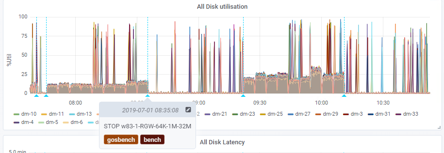
Figure 1. COSBench annotations in the Grafana dashboard
As Figure 1 shows, spikes in disk utilization occurred both inside and outside the COSBench test. These spikes point to the fact that Ceph is performing maintenance tasks and imply that the tests don’t overtax disk performance. One thing to note is that Grafana’s built-in annotations work poorly at large scale. Zooming out to a larger time window displayed only some of the annotations. If larger scale is important, an external annotation source could be used (e.g., a Prometheus query).
Source code for the COSBench annotation tool can be found here.
COSBench run overview 
Once the Grafana annotations were in place, it became easy to see when tests were started and stopped. However, it was still cumbersome to determine when a certain test was executed. The testing team chose to animate a query of the test time from the controller’s website, translate it to the local time zone (or Coordinated Universal Time, UTC), and then set the time window in Grafana. We developed a 17-line Python script that reads out the execution times of the COSBench workloads in the run-history.csv of the controller. It then transforms these date/time objects to the UNIX time (used internally by Grafana) and generates a Grafana link that pads one minute before and after the COSBench execution.
The result is an HTML document where each COSBench test is represented as a direct link to the overview Grafana dashboard. The correct time window is pre-set. Though you may not always want to visit the overview, you can browse to other dashboards while keeping the time window locked when using this link.
Source code for the COSBench run overview tool can be found here.
COSBench-oriented tooling 
When running the 1 billion object test, the testing team had to combine performance metrics from its COSBench tests with information gathered with Prometheus. As such, we needed to collect Prometheus metrics before and after each COSBench run. For example, Prometheus contained the exact total RADOS object count of the cluster at any given time.
To address this need, the team created a small Python 3 tool that would parse the run-history.csv file of the COSBench controller, transform the date/time information to the UNIX timestamp format, and finally execute a query against Prometheus to get the RADOS object count at that precise moment. The output of the tool is a CSV representation of the COSBench workload ID, description, and total object count before and after the workload using semicolons as separators.
Source code for the tool can be found here.
GOSBench distributed Simple Storage Service (S3) performance measurement tool 
COSBench is ideal for testing distributed object storage. At the same time, it has several non-optimal features that forced the test team to spend considerably more time to finish the planned tests. These issues begin with the installation and continue when writing test configurations.
To resolve these issues, the team started to write a new tool, one designed to replace COSBench while making life easier for the testers. We named this new tool GOSBench, because it is written in Golang. Some major differences from COSBench include:
- GOSBench is written in Golang and thus delivered as a static binary.
- Test configurations are implicit rather than explicit.
- Test configurations are written in YAML.
- Performance metrics are available as a Prometheus exporter endpoint.
- Performance metrics automatically exclude preparation steps.
- Fewer system resources are consumed on the load-generating nodes.
- GOSBench can stress the cluster more than COSBench.
While this tool reached a maturity level at which we could have used it for any of our COSBench tests, the team decided to continue using COSBench for this set of tests to have consistent and comparable test results with earlier efforts. In addition, the team ran comparable COSBench and GOSBench tests to see if the performance numbers would match.
The testing team hopes that the community can add some smaller, optional features, ones listed in the TODO.md document. With the help of some early Red Hat internal feedback, the testing team was able to identify certain COSBench use cases that are not easily or obviously approachable with GOSBench. To collect candidates for integration into GOSBench, the team created an issues list in the GitHub repository.
Figures 2 and 3 show screenshots of a sample GOSBench test run. Figure 2 is the output from the GOSBench server, and Figure 3 shows output from one of the seven GOSBench worker nodes used in Red Hat testing. From this output, it’s clear that each worker goes through several phases, specifically that each:
- Initially connects to the server (the worker node receives the S3 connection details and its workload)
- Uses the connection details to prepare for the workload
- Processes the workload
- Re-connects to the server to receive new workloads
The server will ensure that the preparation and performance testing phase synchs across all workers (even when they are not on the same host) and will wait until all workers have finished the current workload before starting more tests.
Source code for GOSBench is available here.

Figure 2. GOSBench server output

Figure 3. GOSBench output from a worker node
GOSBench dashboard 
Unlike many other tools, GOSBench does not output metrics to the command line. Instead, it offers a Prometheus exporter endpoint so it can be scraped. This export functionality is provided by the OpenCensus library, which acts as an HTTP client for the AWS SDK.
To make sense of these metrics and gather similar data, we created a Grafana dashboard. When the Grafana time window is set to the test’s execution time, it displays the same metrics processed for COSBench. Eventually, GOSBench will set Grafana annotations so getting the time window correctly will be easier. For now, the right time window settings are printed to stdout by the GOSBench server. These POST variables can be appended to the Grafana URL. Figure 4 shows a sample dashboard excerpt.
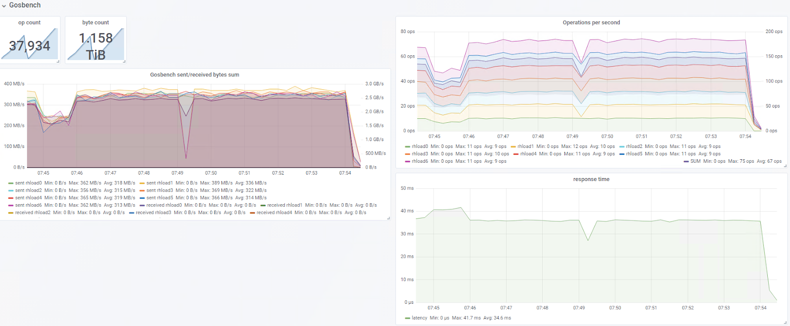
Figure 4. GOSBench Grafana dashboard
Source code for the GOSBench Grafana dashboard can be found here.
COSBench and GOSBench benchmark comparison 
When a new tool is presented, it’s essential to compare it to existing tools for accuracy. For this reason, the team team ran a simple comparison between COSBench and GOSBench. Both tools were tasked to do a 100% read test and a 100% write test on 64KB, 1MB, and 32MB objects for 300 seconds each. The test tools were set to run on all seven RGWs in the test configuration in parallel. Figures 5 and 6 show writing and reading, respectively.

Figure 5. COSBench vs. GOSBench writing to seven RGWs

Figure 6. COSBench vs. GOSBench reading from seven RGWs
From these charts, it’s apparent that the performance metrics for 64KB and 1MB objects are similar for both tools. For the 32MB objects, COSBench reports significantly higher performance metrics than GOSBench. One possible explanation for this disparity is that GOSBench is using multipart uploading and downloading. This feature is not in effect for objects smaller than 5MB and thus would only be visible with the 32MB objects. As of this writing, we’re still looking into this issue.
Conclusion 
The tools developed as a part of Red Hat testing gave testers increased visibility into the details of complicated, large-scale tests. Testers were able to use the Grafana and COSBench tooling to quickly visualize the implications of performance issues, such as disk capacity overloading, and more easily align timing between remote systems under test. While work is ongoing, GOSBench promises to reduce the time needed to set up test installations and write test configurations.